43 excel chart legend labels
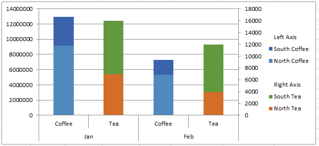
How to Create a Dynamic Chart Range in Excel - Trump Excel This dynamic range is then used as the source data in a chart. As the data changes, the dynamic range updates instantly which leads to an update in the chart. Below is an example of a chart that uses a dynamic chart range. Note that the chart updates with the new data points for May and June as soon as the data in entered. Column Chart with Primary and Secondary Axes - Peltier Tech 28.10.2013 · The second chart shows the plotted data for the X axis (column B) and data for the the two secondary series (blank and secondary, in columns E & F). I’ve added data labels above the bars with the series names, so you can see where the zero-height Blank bars are. The blanks in the first chart align with the bars in the second, and vice versa.
How to Print Labels from Excel - Lifewire Apr 05, 2022 · Connect the Worksheet to the Labels . Before performing the merge to print address labels from Excel, you must connect the Word document to the worksheet containing your list. The first time you connect to an Excel worksheet from Word, you must enable a setting that allows you to convert files between the two programs.
Excel chart legend labels
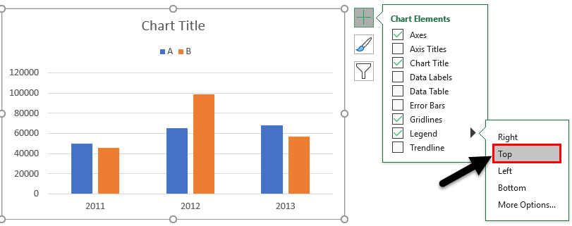
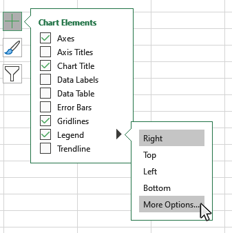
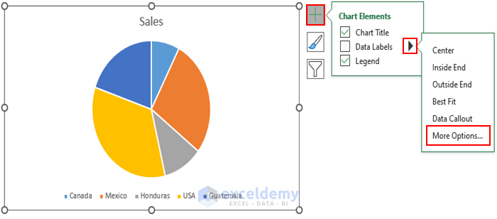
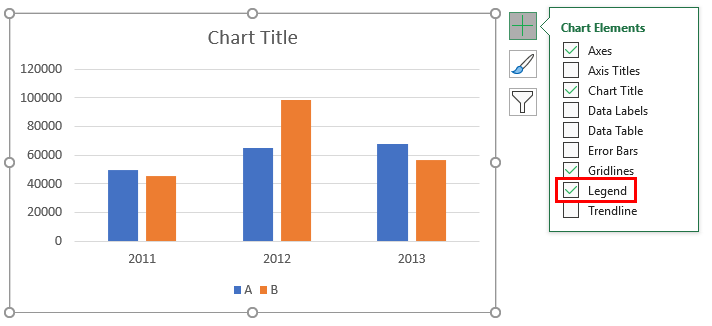
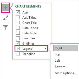
Add and format a chart legend - support.microsoft.com A legend can make your chart easier to read because it positions the labels for the data series outside the plot area of the chart. You can change the position of the legend and customize its colors and fonts. You can also edit the text in the legend and change the order of the entries in the legend. How to Make a Pie Chart in Excel & Add Rich Data Labels to 08.09.2022 · A pie chart is used to showcase parts of a whole or the proportions of a whole. There should be about five pieces in a pie chart if there are too many slices, then it’s best to use another type of chart or a pie of pie chart in order to showcase the data better. In this article, we are going to see a detailed description of how to make a pie chart in excel. Excel Charts - Chart Elements - tutorialspoint.com Now, let us add data Labels to the Pie chart. Step 1 − Click on the Chart. Step 2 − Click the Chart Elements icon. Step 3 − Select Data Labels from the chart elements list. The data labels appear in each of the pie slices. From the data labels on the chart, we can easily read that Mystery contributed to 32% and Classics contributed to 27% ...
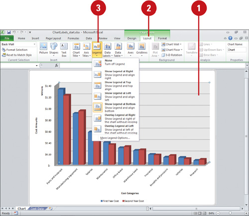
Excel chart legend labels. How to Add Total Data Labels to the Excel Stacked Bar Chart Apr 03, 2013 · For stacked bar charts, Excel 2010 allows you to add data labels only to the individual components of the stacked bar chart. The basic chart function does not allow you to add a total data label that accounts for the sum of the individual components. Fortunately, creating these labels manually is a fairly simply process. Legends in Chart | How To Add and Remove Legends In Excel Chart… Legend is the space located on the plotted area of the chart in excel. It has Legend keys that are connected to the data source. Legend will appear automatically when we insert a chart in excel. We can move the Legend to the top, bottom, right and left of the chart as per requirements by clicking on the “+” symbol and select the Legend ... Show or hide a chart legend or data table If you have space constraints, you may be able to reduce the size of the chart by clearing the Show the legend without overlapping the chart check box. Show or hide a data table Click the chart of a line chart, area chart, column chart, or bar chart in … Pie Chart Examples | Types of Pie Charts in Excel with Examples … But it will be difficult to check the description in the legend and check it on the chart. Now our task is to add the Data series to the PIE chart divisions. Click on the PIE chart so that the chart will get a highlight, as shown below. Right-click and choose the “Add Data Labels “option for additional drop-down options. From that drop-down, select the option “Add Data Callouts ...
Create a Pie Chart in Excel (In Easy Steps) - Excel Easy 6. Create the pie chart (repeat steps 2-3). 7. Click the legend at the bottom and press Delete. 8. Select the pie chart. 9. Click the + button on the right side of the chart and click the check box next to Data Labels. 10. Click the paintbrush icon on the right side of the chart and change the color scheme of the pie chart. Result: 11. Right ... Excel Charts - Chart Elements - tutorialspoint.com Now, let us add data Labels to the Pie chart. Step 1 − Click on the Chart. Step 2 − Click the Chart Elements icon. Step 3 − Select Data Labels from the chart elements list. The data labels appear in each of the pie slices. From the data labels on the chart, we can easily read that Mystery contributed to 32% and Classics contributed to 27% ... How to Make a Pie Chart in Excel & Add Rich Data Labels to 08.09.2022 · A pie chart is used to showcase parts of a whole or the proportions of a whole. There should be about five pieces in a pie chart if there are too many slices, then it’s best to use another type of chart or a pie of pie chart in order to showcase the data better. In this article, we are going to see a detailed description of how to make a pie chart in excel. Add and format a chart legend - support.microsoft.com A legend can make your chart easier to read because it positions the labels for the data series outside the plot area of the chart. You can change the position of the legend and customize its colors and fonts. You can also edit the text in the legend and change the order of the entries in the legend.
Legends in Chart | How To Add and Remove Legends In Excel Chart?
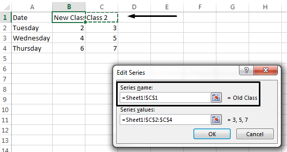
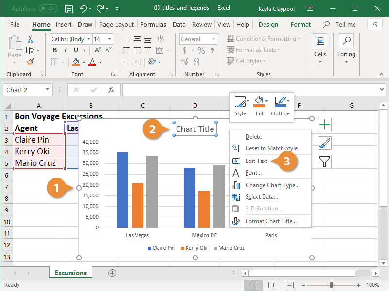
Change legend names
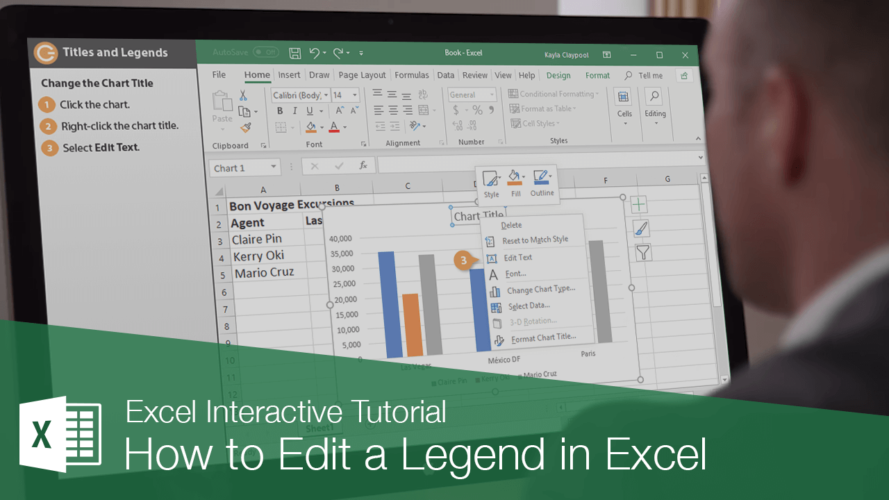
How to Edit a Legend in Excel | CustomGuide

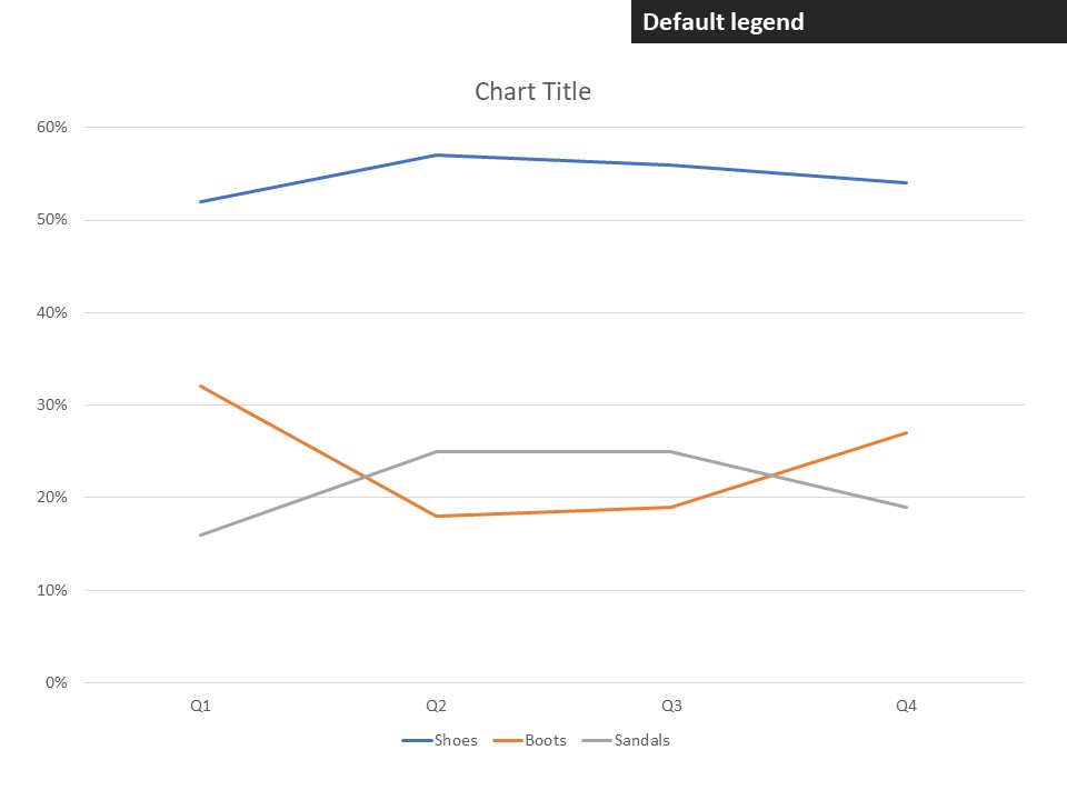
Line charts: Moving the legends next to the line - Microsoft ...

Chart axes, legend, data labels, trendline in Excel - Tech Funda

How to Create a Pie Chart in Excel | Smartsheet
How to Add a Legend to a Chart in Excel - Business Computer ...

Sort legend items in Excel charts – teylyn
Sort legend items in Excel charts – teylyn

Directly Labeling in Excel
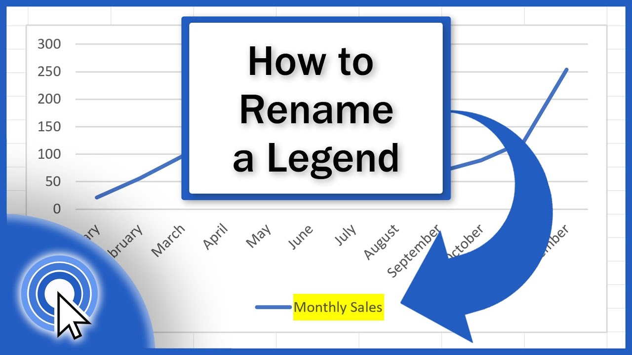
How to Rename a Legend in an Excel Chart (Two Different Ways)

Excel charts: add title, customize chart axis, legend and ...
How-to Group and Categorize Excel Chart Legend Entries ...
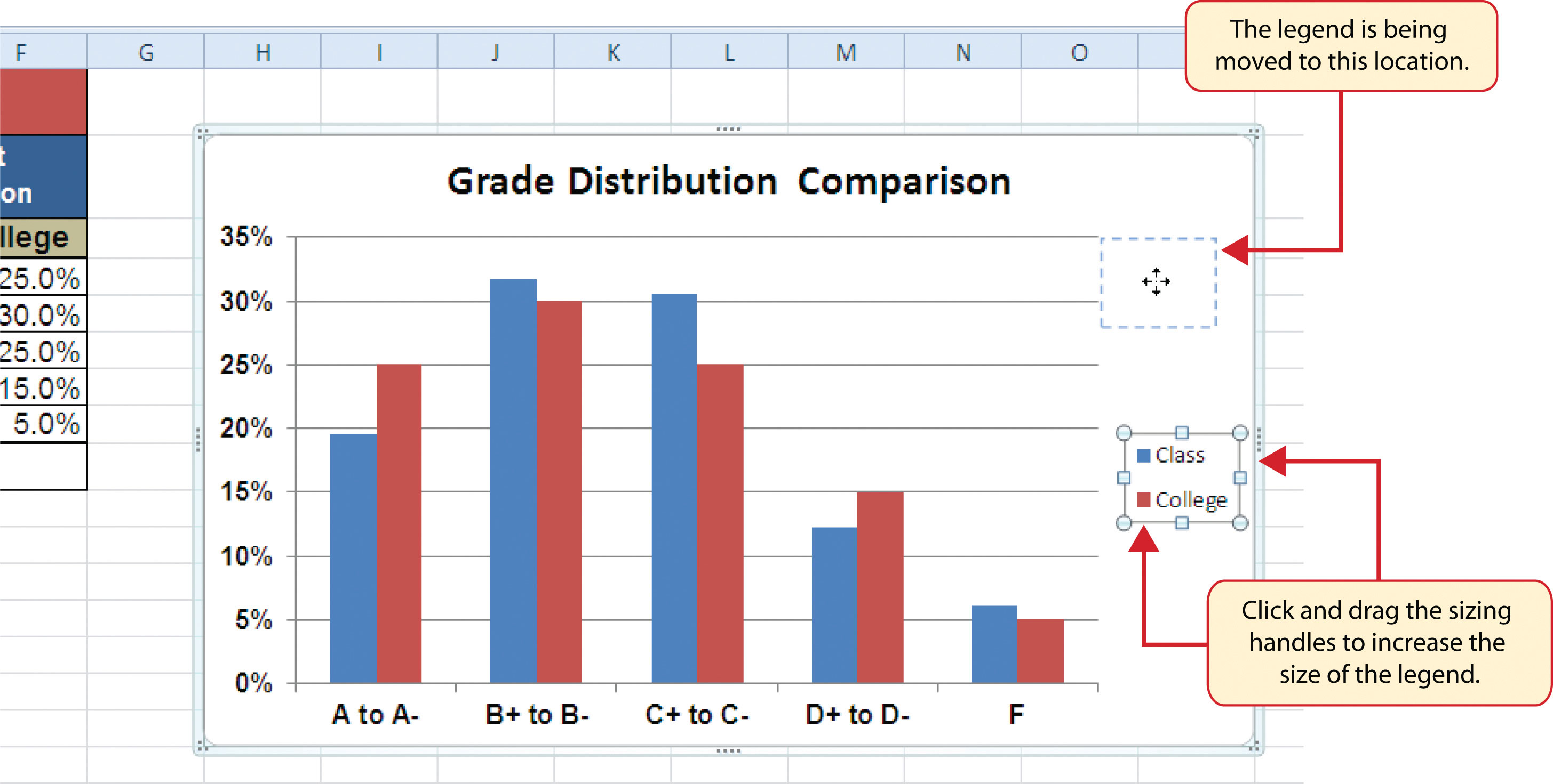
Move and Align Chart Titles, Labels, Legends with the Arrow ...
Change legend names
Formatting Charts
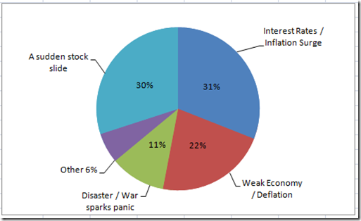
How to Create Pie Chart Legend with Values in Excel - ExcelDemy
Microsoft Excel 2010 : Creating and Modifying Charts ...

Chart Legend in PowerPoint 2010 for Windows
How-to Make a WSJ Excel Pie Chart with Labels Both Inside and ...

How to Make a Pie Chart in Excel - All Things How
Change legend names
Excel Charts with Dynamic Title and Legend Labels (with Steps)
Legends in Chart | How To Add and Remove Legends In Excel Chart?
Add and format a chart legend

Excel charts: add title, customize chart axis, legend and ...

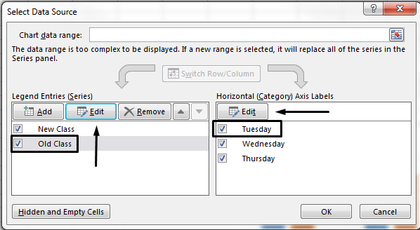
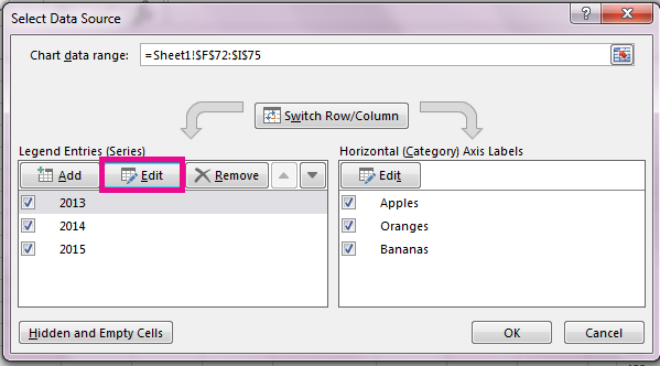
How to Edit Legend Entries in Excel: 9 Steps (with Pictures)
How to Edit a Legend in Excel | CustomGuide
Legend Entry Tricks in Excel Charts - Peltier Tech
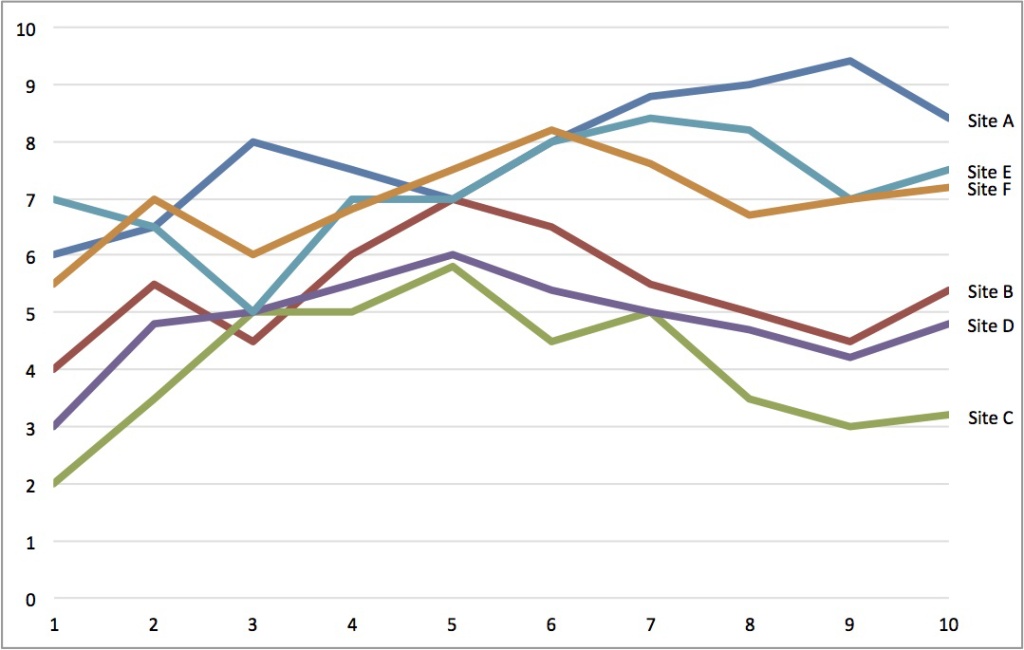
Directly Labeling Excel Charts - PolicyViz

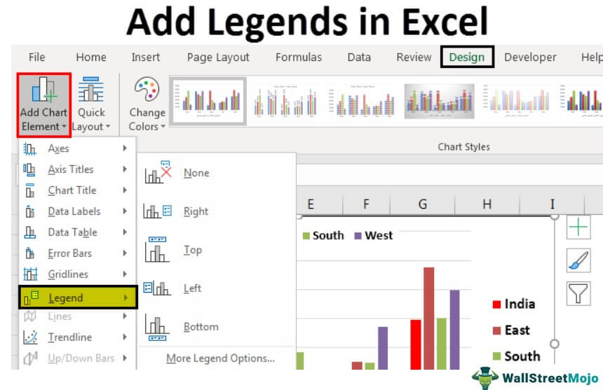
Add a legend to a chart

How to Edit Legend in Excel | Excelchat
Add a legend to a chart
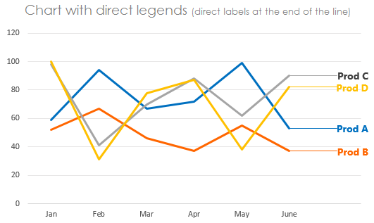
How to add Direct Legends to the Chart - Goodly
Making Excel Chart Legends Better - Example and Download

Change the Chart Legend, Data Labels, and Axis Titles : Chart ...

Directly Labeling Your Line Graphs | Depict Data Studio
7 steps to make a professional looking line graph in Excel or ...
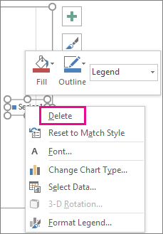
Add and format a chart legend
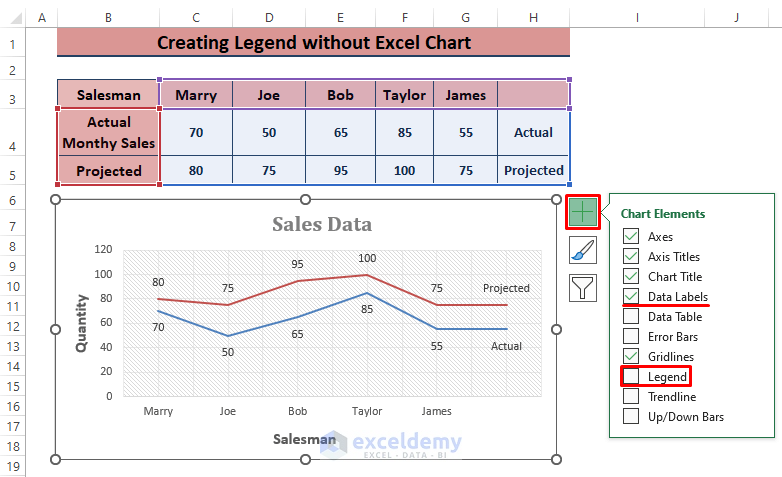
How to Create a Legend in Excel without a Chart (3 Steps ...
Legends in Excel | How to Add legends in Excel Chart?
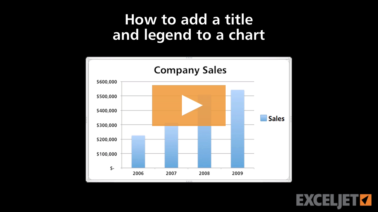
How to add a title and legend to a chart
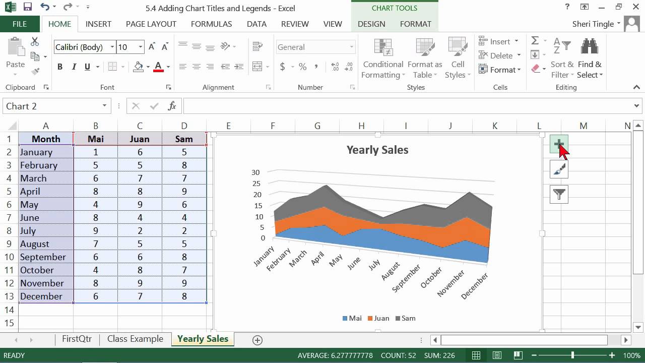
Microsoft Office Excel 2013 Tutorial: Adding Chart Titles and Legends | K Alliance
Post a Comment for "43 excel chart legend labels"