39 change data labels in excel chart
SAS Tutorials: Importing Excel Files into SAS - Kent State University In our case, the dataset we want to import is an Excel file, so select Microsoft Excel Workbook. As you can see, SAS provides you with a large variety of data types to import. Once you've chosen the data source, click Next. Now you need to tell SAS where to find the file you want to import. You can either type the file directory into the text ... How do I add "and" into lists of variable length in Google Sheets? I was able to achieve prepending the "and" to the last word using the ADDRESS (), INDIRECT (), and CONCATENATE () functions but I can't seem to find a way to insert the commas between the first words. I can share with you the file that I have if you'd like. Depending if the number of checkboxes change there might be a way to add the commas.
15 Best Data Visualization Courses, Classes & Training 2022 - CodeSpaces Excel 2013: Charts in Depth By: Dennis Taylor Duration: 3h 46m ... interactive data visualization web apps that plot data in real time and change based on user interaction. It covers the following topics: ... How to add labels and styling to graphs; Introduction to Seaborn - Seaborn is an add-on to Matplotlib. In this module learners explore ...

Change data labels in excel chart
excel - Macro that selects a product from a slicer so pivot charts ... I tried recording a macro that would run that would A. select the product from the slicer and B. set the appropriate primary and secondary axes min and max settings but when I try to run the macro it won't work correctly, in other words it won't just select 2D Design exclusively and apply axes settings. Junk Charts The last number in the series is a negative number and so the real baseline is in the middle of the plot area, where the 0% value is. The following chart shows (left side) the misleading signals sent to readers and (right side) the proper way to consume the data. The degree of distortion is quite extreme. America Works Data Center | U.S. Chamber of Commerce The U.S. Chamber and Chamber Foundation's America Works initiative is mobilizing business and government to swiftly address the crisis. This page captures the trends on job openings, labor force participation, quit rates, and more, for a quick understanding of the state of the workforce. Take a look behind the numbers at what is causing the ...
Change data labels in excel chart. Graph Builder | JMP Interactively create visualizations to explore and describe data. (Examples: dotplots, line plots, box plots, bar charts, histograms, heat maps, smoothers, contour plots, time series plots, interactive geographic maps, mosaic plots) Change number instead of percent in Google Sheet Pie chart - OurTechRoom 1 First click on the piechart 2 Click on 3 dots in the top right corner of the Pie Charts 3 Click on Edit Chart 4 Click on Customize panel 5 Expand the Pie chart section. 6 Under the slice label dropdown select 'value' Now your pie chart looks like this. FORMAT - DAX Guide Dates and times: Use predefined date/time formats or create user-defined date/time formats. The format strings supported as an argument to the DAX FORMAT function are based on the format strings used by Visual Basic (OLE Automation), not on the format strings used by the .NET Framework. Create a bar chart in Excel with start time and duration First, you must select one of the blue-colored bars in your chart > Then right-click on it and choose Format Data Point. A new pane appears on the right side of your Excel sheet. In the Format Data Point pane, you have to click on the symbol and go to Fill > Then choose No fill. Now you can click on the other blue bar and choose No fill.
Resetting the scroll bar in Excel (5 solutions) If you suddenly find yourself in parts of the worksheet you do not wish to populate with data, try this first: Press the Escape key to exit data entry for any cell which is selected. Keep pressing Ctrl + Z to undo any changes made to those cells. Press Ctrl + Up Arrow or Ctrl + Left Arrow to get the selected cell back to a 'normal location'. linkedin-skill-assessments-quizzes/microsoft-project-quiz.md ... - GitHub Change the from Gantt Chart view to Tracking Gantt view. Use the Advanced tab in the Project Options dialog box to enable the Entry Bar. On the View tab on the ribbon, in the Split View group, select Details . Get Digital Help This tutorial shows you how to add a horizontal/vertical line to a chart. Excel allows you to combine two types […] September 23, 2022 . ... Label line chart series. ... Excel Tables simplifies your work with data, adding or removing data, filtering, totals, sorting, enhance readability using cell formatting, cell references, formulas, and ... How to show value instead of aggregate - Power BI If you go to the DATA tab and click on the column name of the table and change the data type of that particular column from Text to Whole Number/Decimal Number and to the number of value you want. Thanks and Regards, Rohit Binnani. Message 10 of 15 78,105 Views 4 Reply Kumail Post Prodigy In response to rohitbinnani 11-28-2017 08:09 AM
Excel Waterfall Chart: How to Create One That Doesn't Suck - Zebra BI Ideally, you would create a waterfall chart the same way as any other Excel chart: (1) click inside the data table, (2) click in the ribbon on the chart you want to insert. ... in Excel 2016 Microsoft decided to listen to user feedback and introduced 6 highly requested charts in Excel 2016, including a built-in Excel waterfall chart. Custom Data Labels With Colors And Symbols In Excel Charts How To ... Select the chart label you want to change. in the formula bar hit = (equals), select the cell reference containing your chart label's data. in this case, the first label is in cell e2. finally, repeat for all your chart laebls. if you are looking for a way to add custom data labels on your excel chart, then this blog post is perfect for you. How to make a Gantt chart in Excel - Ablebits.com Right-click anywhere within the chart plot area (the area with blue and orange bars) and click Select Data to bring up the Select Data Source window again. Make sure the Start Date is selected on the left pane and click the Edit button on the right pane, under Horizontal (Category) Axis Labels. Charts, Graphs & Visualizations by ChartExpo - Google Workspace ChartExpo for Google Sheets has a number of advance charts types that make it easier to find the best chart or graph from charts gallery for marketing reports, agile dashboards, and data analysis: 1. Sankey Diagram 2. Bar Charts 3. Line Graphs (Run Chart) 4. Pie and Donut Charts (Opportunity Charts, Ratio chart) 5.
How to use data labels in a chart
How to Use Excel Pivot Table GetPivotData - Contextures Excel Tips In the formula bar, select the item name, including the quote marks: "Paper" Next, click on cell A4 on the worksheet, where the Paper product name appears The cell reference, A4, will automatically replace the selected text in the formula =GETPIVOTDATA ("Total",$A$3,"Product", A4) Press the Enter key, to complete the formula change

How to Make Pie Chart with Labels both Inside and Outside ...
Format Data | Reporting | DevExpress Documentation Invoke the control's smart tag and click the Format String property's ellipsis button: This invokes the Format String Editor where you can specify the format. Alternatively, you can use the FormatString function within the expression you specified for the report control.

How to Add Data Labels to an Excel 2010 Chart - dummies
Power Apps Excel-Style Editable Table - Part 1 - Matthew Devaney Open Power Apps and create a new Canvas App From Blank called Inventory Count App. Insert a gallery called gal_EditableTable onto the canvas with the 'Inventory Count' SharePoint List as the datasource. Then place 4 text input controls inside the gallery named txt_ItemNumber, txt_Description, txt_Quantity and txt_Location and use this code in each of their Default properties respectively ...

Format Number Options for Chart Data Labels in Excel 2011 for Mac
Transform Values with Table Calculations - Tableau To edit a table calculation: Right-click the measure in the view with the table calculation applied to it and select Edit Table Calculation. In the Table Calculation dialog box that appears, make your changes. When finished, click the X in the top corner of the Table Calculation dialog box to exit it.
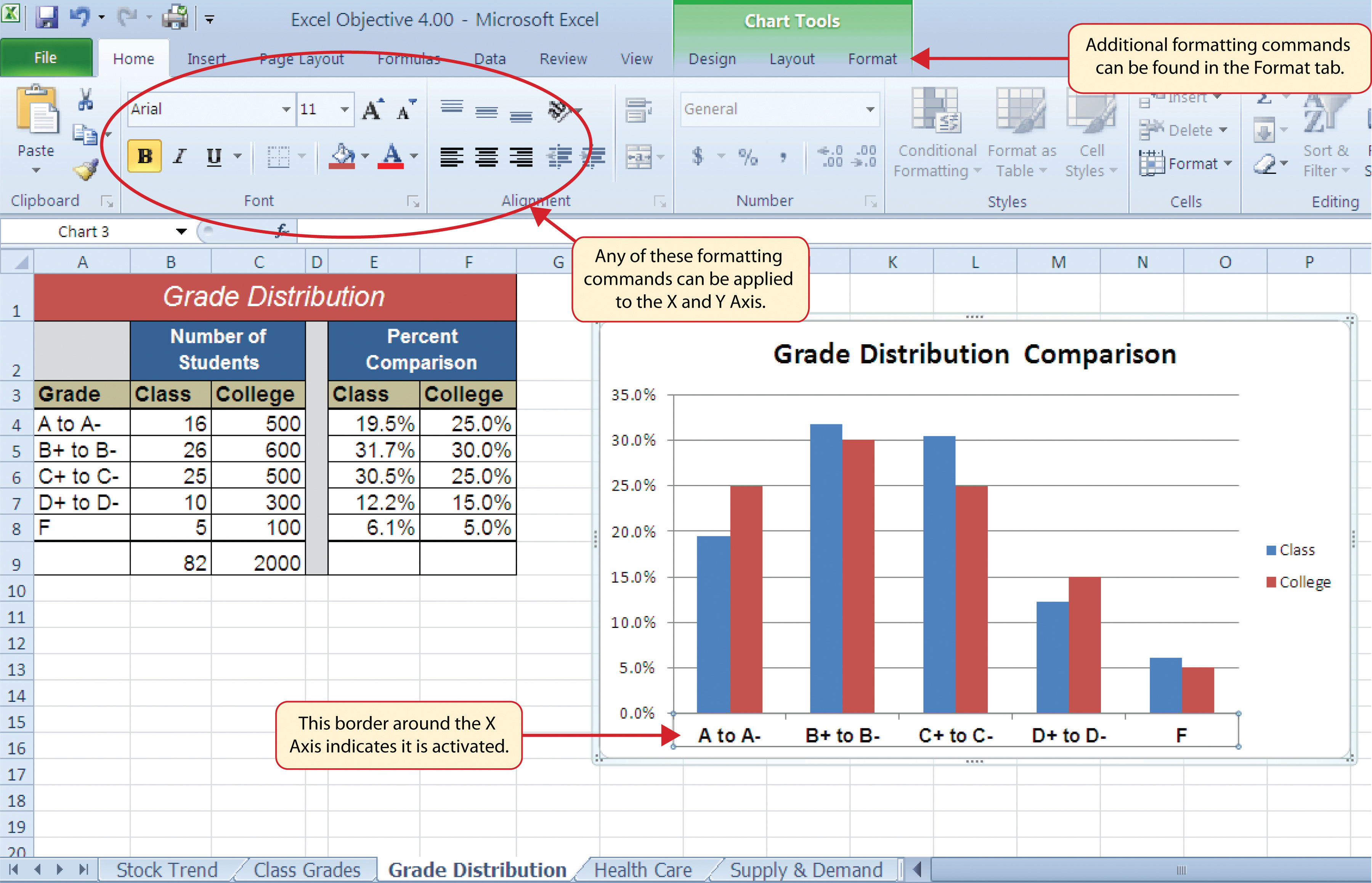
Formatting Charts
Build a bar chart visual in Power BI - Power BI | Microsoft Learn In VS Code, open the [ tsconfig.json] (visual-project-structure.md#tsconfigjson) file and change the name of "files" to "src/barChart.ts". TypeScript Copy "files": [ "src/barChart.ts" ] The tsconfig.json "files" object points to the file where the main class of the visual is located. Your final tsconfig.json file should look like this.
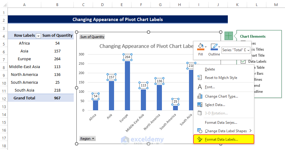
Data Labels in Excel Pivot Chart (Detailed Analysis) - ExcelDemy
Create Custom Data Labels In Excel Charts Youtube In this video i39ll show you how to add data labels to a chart in excel and then change the range that the data labels are linked to- this video covers both w- Home; News; Technology. All; Coding; Hosting; Create Device Mockups in Browser with DeviceMock. Creating A Local Server From A Public Address.

How to Use Cell Values for Excel Chart Labels
Variables Control Charts - I/MR Charts | JMP Data Mining and Predictive Modeling; Quality and Process; Reliability and Survivability; Using SAS from JMP; Download All Guides; Variables Control Charts - I/MR Charts Create Individuals and Moving Range control charts to monitor the performance of a continuous variable over time. Step-by-step guide.
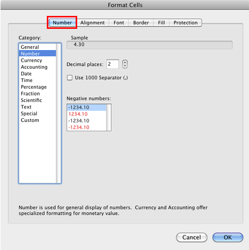
Format Number Options for Chart Data Labels in Excel 2011 for Mac
SAS Tutorials: User-Defined Formats (Value Labels) - Kent State University Recall from the Informats and Formats tutorial that a format in SAS controls how the values of a variable should "look" when printed or displayed. For example, if you have a numeric variable containing yearly income, you could use formats so that the values of those variables are displayed using a dollar sign (without actually modifying the data itself).
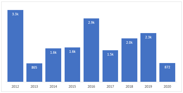
Format Chart Numbers as Thousands or Millions — Excel ...
Learning and resources - Airtable Importing and adding data. Google Sheets importer ; Excel importer ; Creating a new base via CSV import ; How to export a spreadsheet from another source ; Import CSV data into an existing base Updated ; Importing an Airtable CSV into another app ; Can I import my Microsoft Access data into Airtable? Are there file size limits on CSV imports?

How to hide zero data labels in chart in Excel?
How to add titles to Excel charts in a minute - Ablebits.com Click anywhere in the chart. Open the Add Chart Element drop-down menu in the Chart Layouts group on the DESIGN tab. Select the Chart Title option and choose 'None'. Your chart title disappear without a trace. In Excel 2010 you'll find this option if you click on the Chart Title button in the Labels group on the Layout tab. Solution 2

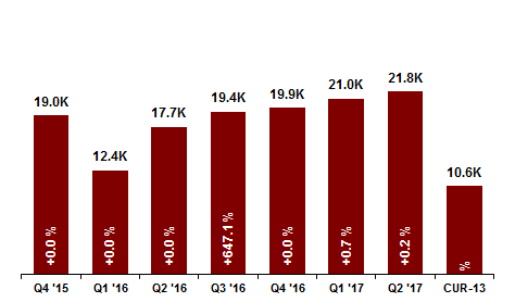
Using the CONCAT function to create custom data labels for an ...
America Works Data Center | U.S. Chamber of Commerce The U.S. Chamber and Chamber Foundation's America Works initiative is mobilizing business and government to swiftly address the crisis. This page captures the trends on job openings, labor force participation, quit rates, and more, for a quick understanding of the state of the workforce. Take a look behind the numbers at what is causing the ...
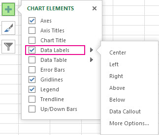
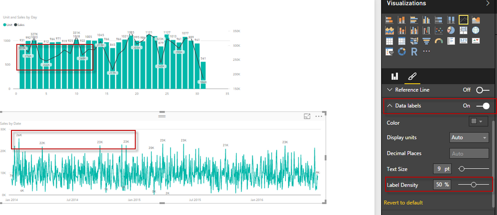
Move data labels
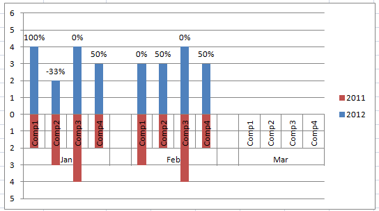
Junk Charts The last number in the series is a negative number and so the real baseline is in the middle of the plot area, where the 0% value is. The following chart shows (left side) the misleading signals sent to readers and (right side) the proper way to consume the data. The degree of distortion is quite extreme.

how to add data labels into Excel graphs — storytelling with data
excel - Macro that selects a product from a slicer so pivot charts ... I tried recording a macro that would run that would A. select the product from the slicer and B. set the appropriate primary and secondary axes min and max settings but when I try to run the macro it won't work correctly, in other words it won't just select 2D Design exclusively and apply axes settings.

Custom data labels in a chart

Add data labels and callouts to charts in Excel 365 ...

How to Make an Excel Pie Chart
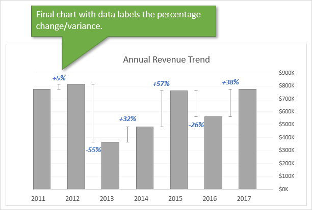
Column Chart That Displays Percentage Change or Variance ...

Adding rich data labels to charts in Excel 2013 | Microsoft ...

Google Workspace Updates: Get more control over chart data ...
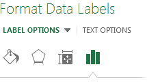
Change the format of data labels in a chart
Excel Clustered Column chart data labels positioning ...
Solved: Data Labels - Microsoft Power BI Community

Change the format of data labels in a chart

Custom data labels in a chart

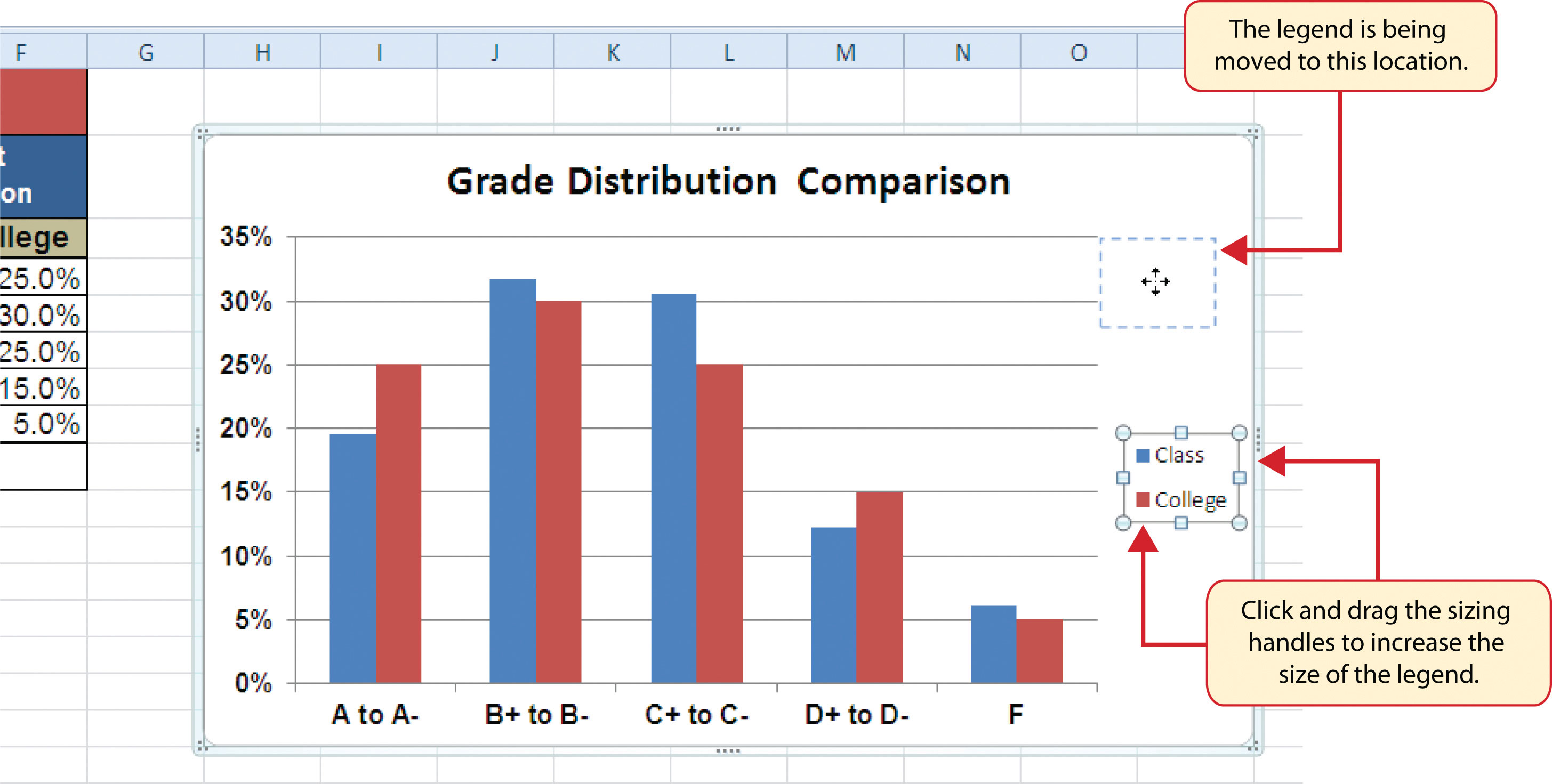
Excel charts: add title, customize chart axis, legend and ...
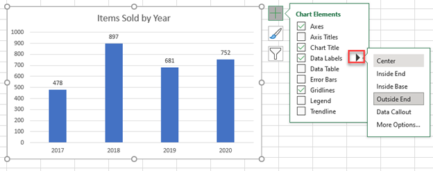
Add / Move Data Labels in Charts – Excel & Google Sheets ...

Creating Graphs in Excel 2013

How to Change Excel Chart Data Labels to Custom Values?

Excel charts: add title, customize chart axis, legend and ...

Adding rich data labels to charts in Excel 2013 | Microsoft ...

Change the format of data labels in a chart

Highlight a Specific Data Label in an Excel Chart - Peltier Tech
Add % Difference Data Labels to Excel Horizontal Tornado ...
Formatting Charts

How to Add Total Data Labels to the Excel Stacked Bar Chart ...

Office: Display Data Labels in a Pie Chart

How to Add Data Labels to your Excel Chart in Excel 2013

Is it possible to conditionally format Data Labels on a ...

Adding Data Labels to Your Chart (Microsoft Excel)
Post a Comment for "39 change data labels in excel chart"