44 how to add percentage and category name data labels in excel

Custom Chart Data Labels In Excel With Formulas - How To Excel At Excel Follow the steps below to create the custom data labels. Select the chart label you want to change. In the formula-bar hit = (equals), select the cell reference containing your chart label's data. In this case, the first label is in cell E2. Finally, repeat for all your chart laebls. How to set and format data labels for Excel charts in C# - E-ICEBLUE It's worthy of mention that Spire.XLS also supports data labels which are widely used to quickly identify a data series in a chart. In label options, we could set whether label contains series name, category name, value, percentages (pie chart) and legend key.

Add or remove data labels in a chart - support.microsoft.com Add data labels to a chart Click the data series or chart. To label one data point, after clicking the series, click that data point. In the upper right corner, next to the chart, click Add Chart Element > Data Labels. To change the location, click the arrow, and choose an option.

How to add percentage and category name data labels in excel

How to show data label in "percentage" instead of - answers.microsoft.com Select Format Data Labels Select Number in the left column Select Percentage in the popup options In the Format code field set the number of decimal places required and click Add. (Or if the table data in in percentage format then you can select Link to source.) Click OK Regards, OssieMac Report abuse 8 people found this reply helpful · Excel tutorial: How to use data labels When you check the box, you'll see data labels appear in the chart. If you have more than one data series, you can select a series first, then turn on data labels for that series only. You can even select a single bar, and show just one data label. In a bar or column chart, data labels will first appear outside the bar end. How to show percentages in stacked column chart in Excel? - ExtendOffice Add percentages in stacked column chart 1. Select data range you need and click Insert > Column > Stacked Column. See screenshot: 2. Click at the column and then click Design > Switch Row/Column. 3. In Excel 2007, click Layout > Data Labels > Center . In Excel 2013 or the new version, click Design > Add Chart Element > Data Labels > Center. 4.

How to add percentage and category name data labels in excel. excel - How can I add chart data labels with percentage? - Stack Overflow I want to add chart data labels with percentage by default with Excel VBA. Here is my code for creating the chart: Private Sub CommandButton2_Click() ActiveSheet.Shapes.AddChart.Select ActiveChart. Pivot Chart Data Label Help Needed - Microsoft Community Open the Excel file with Pivot Chart and enabled with Data Labels> Click on the Labels displayed in the Chart> Right-click> Click Format Data Labels> Label Options> Number> In the Category, select the format as per your requirement. Here is the reference article: Change the format of data labels in a chart. Change the format of data labels in a chart - support.microsoft.com To get there, after adding your data labels, select the data label to format, and then click Chart Elements > Data Labels > More Options. To go to the appropriate area, click one of the four icons ( Fill & Line, Effects, Size & Properties ( Layout & Properties in Outlook or Word), or Label Options) shown here. Multiple Data Labels on bar chart? - Excel Help Forum Select A1:D4 and insert a bar chart. Select 2 series and delete it. Select 2 series, % diff base line, and move to secondary axis. Adjust series 2 data references, Value from B2:D2. Category labels from B4:D4. Apply data labels to series 2 outside end. select outside end data labels and change from Values to Category Name.

Tips for Analyzing Categorical Data in Excel - The Excel Club There are only a few steps involved in setting up a pivot table. First, click on any cell within the data set. Then press Atl +N+V. This will open the Create Pivot Table dialogue box. Alternatively, select Pivot table from the Insert Ribbon. This will also open the Pivot Table dialogue Box. Next, select a table or range of data that is to be ... Data Bars in Excel (Examples) | How to Add Data Bars in Excel? - EDUCBA In order to show only bars, you can follow the below steps. Step 1: Select the number range from B2:B11. Step 2: Go to Conditional Formatting and click on Manage Rules. Step 3: As shown below, double click on the rule. Step 4: Now, in the below window, select Show Bars Only and then click OK. Add a DATA LABEL to ONE POINT on a chart in Excel - Excel Quick Help Steps shown in the video above: Click on the chart line to add the data point to. All the data points will be highlighted. Click again on the single point that you want to add a data label to. Right-click and select ' Add data label ' This is the key step! Right-click again on the data point itself (not the label) and select ' Format data label '. How to show percentage in Excel - Ablebits To do this, open the Format Cells dialog either by pressing Ctrl + 1 or right-clicking the cell and selecting Format Cells… from the context menu. Make sure the Percentage category is selected and specify the desired number of decimal places in the Decimal places box. When done, click the OK button to save your settings.

How to Add Data Labels to an Excel 2010 Chart - dummies On the Chart Tools Layout tab, click Data Labels→More Data Label Options. The Format Data Labels dialog box appears. You can use the options on the Label Options, Number, Fill, Border Color, Border Styles, Shadow, Glow and Soft Edges, 3-D Format, and Alignment tabs to customize the appearance and position of the data labels. Excel.ChartDataLabels class - Office Add-ins | Microsoft Docs The request context associated with the object. This connects the add-in's process to the Office host application's process. Specifies the format of chart data labels, which includes fill and font formatting. Specifies the horizontal alignment for chart data label. See Excel.ChartTextHorizontalAlignment for details. Solved: change data label to percentage - Power BI pick your column in the Right pane, go to Column tools Ribbon and press Percentage button do not hesitate to give a kudo to useful posts and mark solutions as solution LinkedIn Message 2 of 7 1,653 Views 1 Reply MARCreading Regular Visitor In response to az38 06-09-2020 09:03 AM Hi @az38, Thanks for your help! How to Add Total Data Labels to the Excel Stacked Bar Chart Step 4: Right click your new line chart and select "Add Data Labels" Step 5: Right click your new data labels and format them so that their label position is "Above"; also make the labels bold and increase the font size. Step 6: Right click the line, select "Format Data Series"; in the Line Color menu, select "No line"

Pie Chart Examples | Types of Pie Charts in Excel with Examples

Format Number Options for Chart Data Labels in Excel 2011 ... - Indezine Figure 1: Chart with Data Values added as Data Labels. Follow these steps to learn how to format the values used in Data Labels within Excel 2011: Select the chart -- then select the Charts tab which appears on the Ribbon, as shown highlighted in red within Figure 2. Within the Charts tab, click the Edit button (highlighted in blue within ...

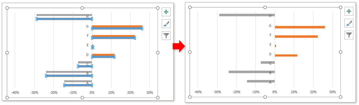
Quickly create a positive negative bar chart in Excel

How to show values in data labels of Excel Pareto Chart when chart is ... 2) Move Value data series to 2nd Axis 3) Change Value data series Fill from Automatic to No Fill 4) Change 2nd Vertical Axis Labels to None 5) Add Data Labels to Value data series Hope this helps. Steve=True D dendres New Member Joined Aug 1, 2015 Messages 14 Aug 3, 2015 #3 Hi Steve=True, Thank you for the help.

Art of Charts: Bubble grid charts: an alternative to stacked bar/column charts with lots of data ...

How to Add Percentage Axis to Chart in Excel - OfficeTuts Excel To do this, we will select the whole table again, and then go to Insert >> Charts >> 2-D Columns: To show percentages on a second axis, we first need to click anywhere on the orange bars that we have on our graph (this is not easy in this example as they are rather small). Once we do, we will right-click on it, and then select Format Data Series:

Excel Questions 1. Chart 1- Rename the line chart | Chegg.com

Chart.ApplyDataLabels method (Excel) | Microsoft Docs Syntax expression. ApplyDataLabels ( Type, LegendKey, AutoText, HasLeaderLines, ShowSeriesName, ShowCategoryName, ShowValue, ShowPercentage, ShowBubbleSize, Separator) expression A variable that represents a Chart object. Parameters Example This example applies category labels to series one on Chart1. VB Copy Charts ("Chart1").SeriesCollection (1).

How to Create a Pie Chart in Excel | Smartsheet

How to Change Excel Chart Data Labels to Custom Values? - Chandoo.org First add data labels to the chart (Layout Ribbon > Data Labels) Define the new data label values in a bunch of cells, like this: Now, click on any data label. This will select "all" data labels. Now click once again. At this point excel will select only one data label.

How to Create a Pie Chart in Excel | Smartsheet

How to create a chart with both percentage and value in Excel? In the Format Data Labels pane, please check Category Name option, and uncheck Value option from the Label Options, and then, you will get all percentages and values are displayed in the chart, see screenshot: 15.

Changing Axis Labels in PowerPoint 2011 for Mac

Excel charts: add title, customize chart axis, legend and data labels To add a label to one data point, click that data point after selecting the series. Click the Chart Elements button, and select the Data Labels option. For example, this is how we can add labels to one of the data series in our Excel chart: For specific chart types, such as pie chart, you can also choose the labels location.

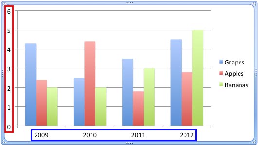
4.1 Choosing a Chart Type – Beginning Excel, First Edition

How to Customize Your Excel Pivot Chart Data Labels - dummies The Data Labels command on the Design tab's Add Chart Element menu in Excel allows you to label data markers with values from your pivot table. When you click the command button, Excel displays a menu with commands corresponding to locations for the data labels: None, Center, Left, Right, Above, and Below. None signifies that no data labels ...

Share :