41 excel chart horizontal axis labels
› charts › axis-labelsHow to add Axis Labels (X & Y) in Excel & Google Sheets Type in your new axis name; Make sure the Axis Labels are clear, concise, and easy to understand. Dynamic Axis Titles. To make your Axis titles dynamic, enter a formula for your chart title. Click on the Axis Title you want to change; In the Formula Bar, put in the formula for the cell you want to reference (In this case, we want the axis title ... Excel Waterfall Chart: How to Create One That Doesn't Suck The first and last columns should be Total (start on the horizontal axis) and to set them as such, we have to double-click on each of them to open the Format Data Point task pane, and check the Set as total box. You can also right click the data point and select Set as Total from the list of menu options. Finally, we have our waterfall chart: 2.
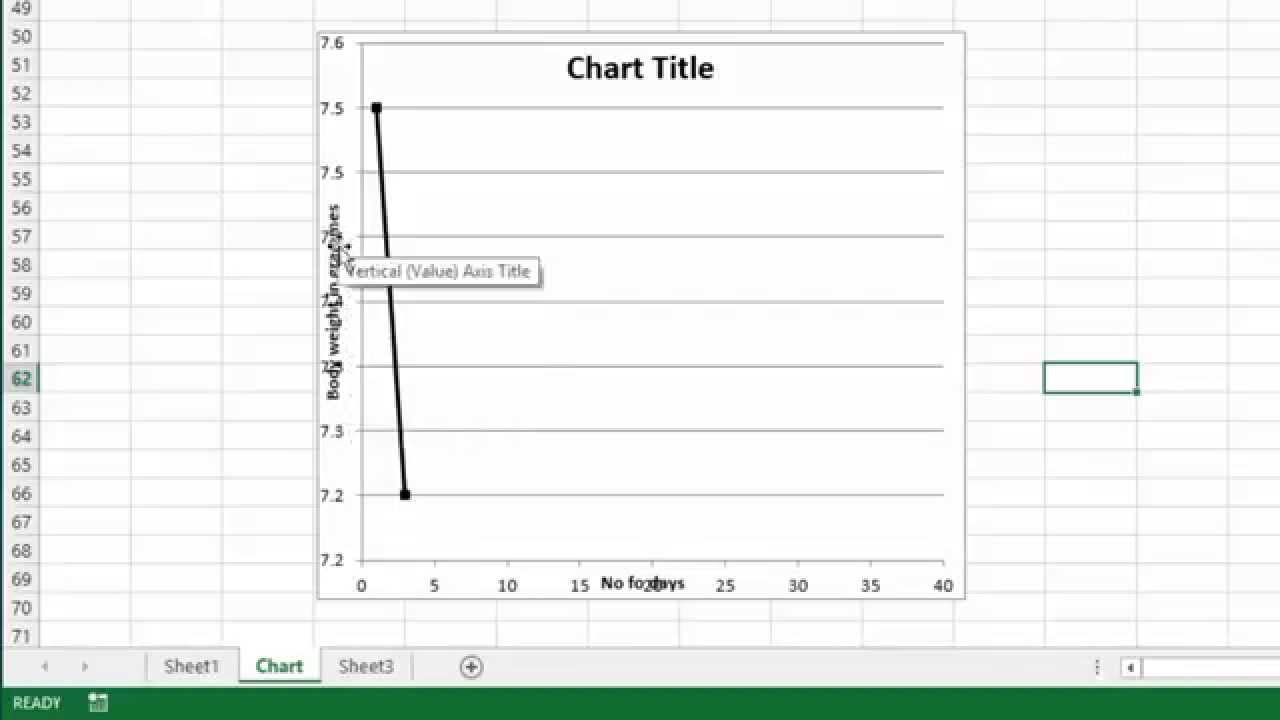
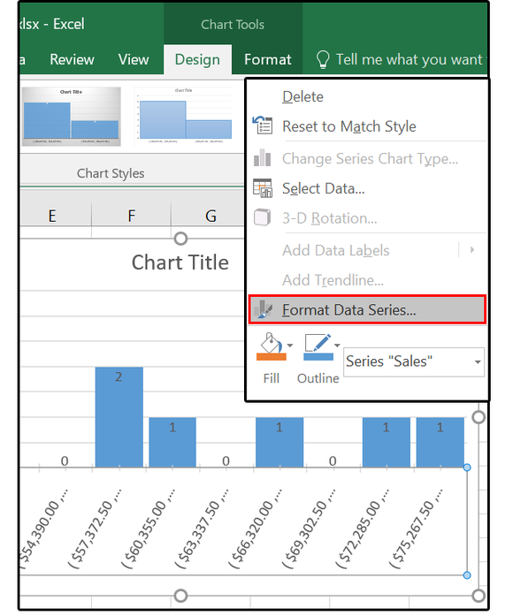
Format Chart Axis in Excel - Axis Options Right-click on the Vertical Axis of this chart and select the "Format Axis" option from the shortcut menu. This will open up the format axis pane at the right of your excel interface. Thereafter, Axis options and Text options are the two sub panes of the format axis pane. Formatting Chart Axis in Excel - Axis Options : Sub Panes
Excel chart horizontal axis labels
Chart two columns of data on the horizontal axis Chart two columns of data on the horizontal axis. When I download my blood pressure data from my monitor I get one column for dates and another column for times within each date. I'm trying to get a chart with data points for each date and time. I don't know to create a formula for the horizontal axis which combine column A (date) and Column B ... How to make shading on Excel chart and move x axis labels to the bottom ... In the text options for the horizontal axis, specify a custom angle of -45 degress (or whichever value you prefer): For the yellow shading, add a series with constant value -80, and a series with constant value -20. In the Change Chart Type dialog, change the chart type for the new series to Stacked Area. › excel-chart-verticalExcel Chart Vertical Axis Text Labels - My Online Training Hub Apr 14, 2015 · Let’s cull some of those axes and format the chart: Click on the top horizontal axis and delete it. Hide the left hand vertical axis: right-click the axis (or double click if you have Excel 2010/13) > Format Axis > Axis Options: Set tick marks and axis labels to None
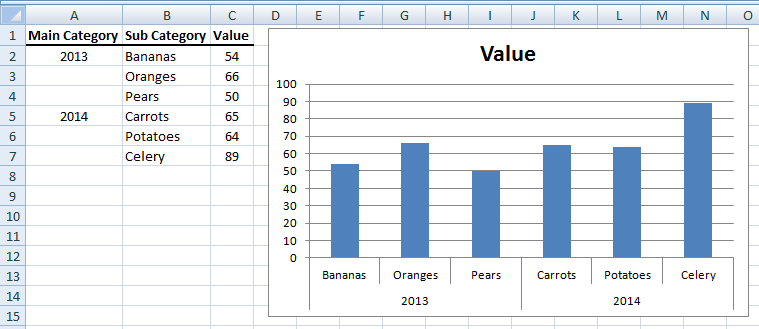
Excel chart horizontal axis labels. Excel: How to Create a Bubble Chart with Labels - Statology Step 3: Add Labels. To add labels to the bubble chart, click anywhere on the chart and then click the green plus "+" sign in the top right corner. Then click the arrow next to Data Labels and then click More Options in the dropdown menu: In the panel that appears on the right side of the screen, check the box next to Value From Cells within ... excel - Line chart with grouped values on horizontal axis - Stack Overflow What you have to do is to unmerge those cells and place the label in an appropriately "centered" row, e.g. A4="Monday" and A11="Tuesday". This should produce the axis labels you've described. You can format the cell borders to make the table look exactly the same as your post. - PeterT May 17 at 17:20 Add a comment Excel Charts with Shapes for Infographics - My Online Training Hub How to Build Excel Charts with Shapes. Start by inserting a regular column chart. Then insert the shape you want to use. Make sure it's roughly the same size as the largest column in your chart. CTRL+C to copy the Shape > Select the columns in the chart > CTRL+V to paste the shape. Tip: add data labels and remove the gridlines and vertical axis. How to group (two-level) axis labels in a chart in Excel? The Pivot Chart tool is so powerful that it can help you to create a chart with one kind of labels grouped by another kind of labels in a two-lever axis easily in Excel. You can do as follows: 1. Create a Pivot Chart with selecting the source data, and: (1) In Excel 2007 and 2010, clicking the PivotTable > PivotChart in the Tables group on the ...
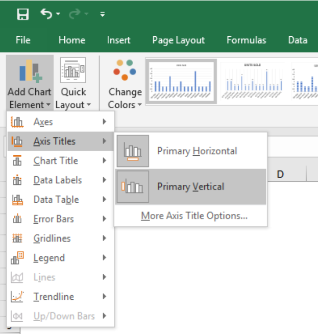
How to Add Axis Titles in a Microsoft Excel Chart Select the chart and go to the Chart Design tab. Click the Add Chart Element drop-down arrow, move your cursor to Axis Titles, and deselect "Primary Horizontal," "Primary Vertical," or both. In Excel on Windows, you can also click the Chart Elements icon and uncheck the box for Axis Titles to remove them both. Change Primary Axis in Excel - Excel Tutorials Most Excel charts have two types of primary axes: the category or x-axis and the value or y-axis. The category axis is the horizontal axis and is usually located at the bottom of the chart. The value axis is the vertical axis and is normally located on the left side of the chart. › charts › move-horizontalMove Horizontal Axis to Bottom – Excel & Google Sheets Moving X Axis to the Bottom of the Graph. Click on the X Axis; Select Format Axis . 3. Under Format Axis, Select Labels. 4. In the box next to Label Position, switch it to Low. Final Graph in Excel. Now your X Axis Labels are showing at the bottom of the graph instead of in the middle, making it easier to see the labels. Format Chart Axis in Excel – Axis Options 14/12/2021 · Formatting a Chart Axis in Excel includes many options like Maximum / Minimum Bounds, Major / Minor units, Display units, Tick Marks, Labels, Numerical Format of the axis values, Axis value/text direction, and more. However, there are a lot more formatting options for the chart axis, in this blog, we will be working with the axis options and ...
How to Adjust the Width or Height of Chart Margins on an Excel ... Between the two borders is where a lot of information goes. Specifically between the left-hand chart area border and plot area border is where the vertical axis values and labels go. Similar for right hand side if there is a secondary axis and for the bottom where horizontal axis values and labels go. Chart.Axes method (Excel) | Microsoft Docs This example adds an axis label to the category axis on Chart1. VB. With Charts ("Chart1").Axes (xlCategory) .HasTitle = True .AxisTitle.Text = "July Sales" End With. This example turns off major gridlines for the category axis on Chart1. VB. superuser.com › questions › 1195816Excel Chart not showing SOME X-axis labels - Super User Apr 05, 2017 · In Excel 2013, select the bar graph or line chart whose axis you're trying to fix. Right click on the chart, select "Format Chart Area..." from the pop up menu. A sidebar will appear on the right side of the screen. On the sidebar, click on "CHART OPTIONS" and select "Horizontal (Category) Axis" from the drop down menu. Change the scale of the horizontal (category) axis in a chart The horizontal (category) axis, also known as the x axis, of a chart displays text labels instead of numeric intervals and provides fewer scaling options than are available for a vertical (value) axis, also known as the y axis, of the chart. However, you can specify the following axis options: Interval between tick marks and labels
Fixing Your Excel Chart When the Multi-Level Category Label Option is Missing. - Excel Dashboard ...
› documents › excelHow to group (two-level) axis labels in a chart in Excel? The Pivot Chart tool is so powerful that it can help you to create a chart with one kind of labels grouped by another kind of labels in a two-lever axis easily in Excel. You can do as follows: 1. Create a Pivot Chart with selecting the source data, and: (1) In Excel 2007 and 2010, clicking the PivotTable > PivotChart in the Tables group on the ...
35 How To Label The Axis In Excel - Label Design Ideas 2020
How to make a quadrant chart using Excel - Basic Excel Tutorial Go to the 'Label Options' tab and check the 'Value from cells' option. Select all the names and click OK. Uncheck the 'Y Value' box and under 'Label Position,' select 'Above. 7. Add the Axis titles. Select the chart and go to the 'Design' tab. Choose 'Add Chart Element' and click 'Axis Titles.' Pick both 'Primary Horizontal' and 'Primary Vertical.'

Stagger long axis labels and make one label stand out in an Excel column chart | Think Outside ...
How to Create a Mekko Chart (Marimekko) in Excel - Quick Guide Here are the steps to create a Mekko chart: #1: Set up a helper table and add data. #2: Append the helper table with zeros. #3: Apply a custom number format. #4: Calculate and add segment values. #5: Set up the horizontal axis values. #6: Calculate midpoints. #7: Add labels for rows and columns.
33 How To Label Axis On Excel Mac 2016 - Labels 2021
Excel Chart not showing SOME X-axis labels - Super User 05/04/2017 · On the sidebar, click on "CHART OPTIONS" and select "Horizontal (Category) Axis" from the drop down menu. Four icons will appear below the menu bar. The right most icon looks like a bar graph. Click that. A navigation bar with several twistys will appear below the icon ribbon. Click on the "LABELS" twisty. You can play with the options under here to get your X …

Making Horizontal Dot Plot or Dumbbell Charts in Excel - How To - PakAccountants.com
Two-Level Axis Labels (Microsoft Excel) Excel automatically recognizes that you have two rows being used for the X-axis labels, and formats the chart correctly. Since the X-axis labels appear beneath the chart data, the order of the label rows is reversed—exactly as mentioned at the first of this tip. (See Figure 1.) Figure 1. Two-level axis labels are created automatically by Excel.

Charting in Excel - Adding Axis Labels - YouTube
How to Add Axis Label to Chart in Excel - Sheetaki Select the chart that you want to add an axis label. Next, head over to the Chart tab. Click on the Axis Titles. Navigate through Primary Horizontal Axis Title > Title Below Axis. An Edit Title dialog box will appear. In this case, we will input "Month" as the horizontal axis label. Next, click OK.
34 How To Label Axis In Excel - Labels For You
Excel Charts - Chart Elements - Tutorials Point Axis titles give the understanding of the data of what the chart is all about. You can add axis titles to any horizontal, vertical, or the depth axes in the chart. You cannot add axis titles to charts that do not have axes (Pie or Doughnut charts). To add Axis Titles, Step 1 − Click on the chart. Step 2 − Click the Chart Elements icon.
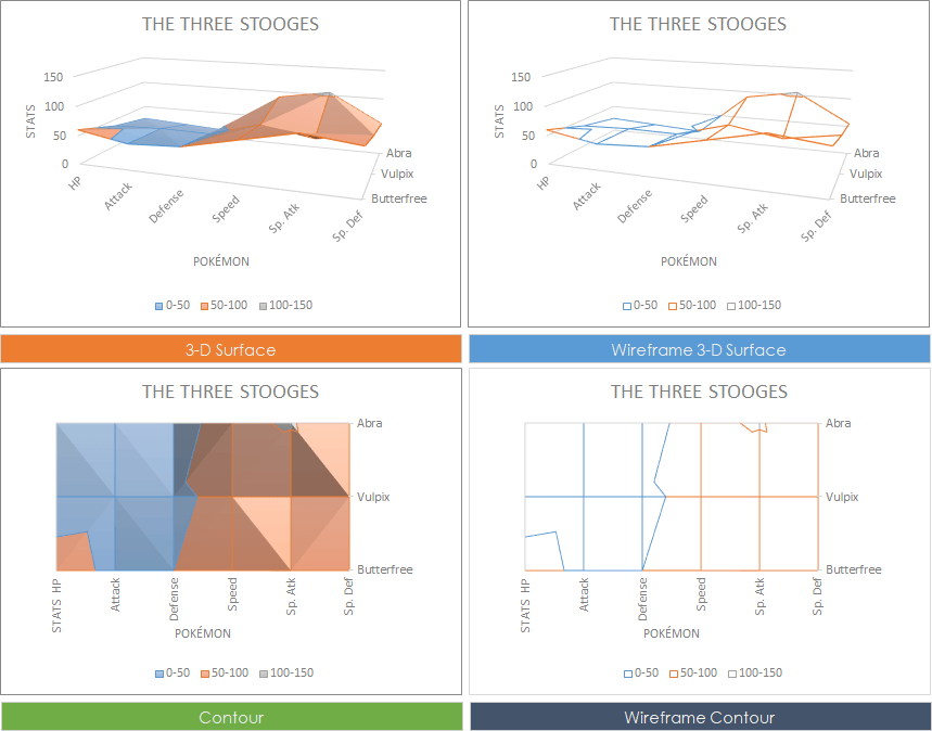
Surface Chart in Excel
Broken Y Axis in an Excel Chart - Peltier Tech 18/11/2011 · I’ve also set the labels of the primary horizontal axis (center of the chart) to No Labels, because they are redundant and clutter up the chart. The primary and secondary axis scales conveniently have the right spacing so that the primary horizontal gridlines work for the secondary axis as well. Now I’ve applied the same fill colors to the secondary axis columns as …
Moving X-axis labels at the bottom of the chart below negative values in Excel - PakAccountants.com
Use defined names to automatically update a chart range - Office On the Insert tab, click a chart, and then click a chart type. Click the Design tab, click the Select Data in the Data group. Under Legend Entries (Series), click Edit. In the Series values box, type =Sheet1!Sales, and then click OK. Under Horizontal (Category) Axis Labels, click Edit.

How to Insert Axis Labels In An Excel Chart | Excelchat
Excel Chart Vertical Axis Text Labels • My Online Training Hub 14/04/2015 · Let’s cull some of those axes and format the chart: Click on the top horizontal axis and delete it. Hide the left hand vertical axis: right-click the axis (or double click if you have Excel 2010/13) > Format Axis > Axis Options: Set tick marks and axis labels to None

Excel - 2-D Bar Chart - Change horizontal axis labels - Super User
support.microsoft.com › en-us › topicChange the scale of the horizontal (category) axis in a chart The horizontal (category) axis, also known as the x axis, of a chart displays text labels instead of numeric intervals and provides fewer scaling options than are available for a vertical (value) axis, also known as the y axis, of the chart. However, you can specify the following axis options: Interval between tick marks and labels

31 How To Label Chart Axis In Excel - Labels For Your Ideas
Date Axis in Excel Chart is wrong • AuditExcel.co.za If you right click on the horizontal axis and choose to Format Axis, you will see that under Axis Type it has 3 options being Automatic, text or date. As we have entered valid dates in the data the Automatic chooses dates and therefore you get the option in the second box. If Excel sees valid dates it will allow you to control the scale into ...
How to Make a Bar Chart - ExcelNotes
How to create Marimekko Chart (Mekko Chart) in Excel - Quick Guide Steps to create a Marimekko chart in Excel: #1: Prepare data and create a helper table. #2: Append the helper table with zeros. #3: Use custom number format in the helper column. #4: Calculate and add segment values. #5: Set up the horizontal axis values.
Resize the Plot Area in Excel Chart - Titles and Labels Overlap - YouTube
Histogram Chart in Excel - Insert, Format, Bins - Excel Unlocked Click on the chart and on the ribbon, find the Format tab. In the Current Selection group, mark the Horizontal Axis. Press ctrl+1. This opens the Format Axis pane for the Horizontal Axis. Navigate to the Axis Options tab. Mark the Bin Width as 3. Set the Overflow Bin as 10 ( It is the Upper Value of the Last Interval )
How to Insert Axis Labels In An Excel Chart | Excelchat
Modifying Axis Scale Labels (Microsoft Excel) Create your chart as you normally would. Double-click the axis you want to scale. You should see the Format Axis dialog box. (If double-clicking doesn't work, right-click the axis and choose Format Axis from the resulting Context menu.) Make sure the Scale tab is displayed. (See Figure 2.) Figure 2. The Scale tab of the Format Axis dialog box.

How to label chart axes in Excel: add axis titles to graphs - PC Advisor
Excel - 2-D Bar Chart - Change horizontal axis labels - Super User And then go to Chart Design tab > Change Chart Type > All Charts tab > Combo, set different chart types as below. Slect the chart, locate to Chart Design > Add Chart Element > Axes > Choose all Horizontal and Vertical axes to show. Please choose the Secondary Horizontal, set it across 0. Choose the Secondary Vertical, set it across 0 too.
Excel 2016 charts: How to use the new Pareto, Histogram, and Waterfall formats | PCWorld
How to Create and Customize a Pareto Chart in Microsoft Excel Go to the Insert tab and click the "Insert Statistical Chart" drop-down arrow. Select "Pareto" in the Histogram section of the menu. Remember, a Pareto chart is a sorted histogram chart. And just like that, a Pareto chart pops into your spreadsheet. You'll see your categories as the horizontal axis and your numbers as the vertical axis.
Post a Comment for "41 excel chart horizontal axis labels"